1. Practical guide of the industrial fan
Once an air motion is established, a pressure drop is generated, as well as, when an electrical current is established, a voltage drop is generated. In other words, there is air motion between two points if there is a difference of pressure between this two points, as well as, the current is established when there is an electric potential difference
Type of fans
The fan is therefore a “pressure generator” able to override the pressure drop and to motion the air.
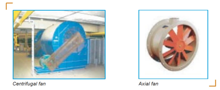
Theoretically, any kind of fan is able to produce any requested pressure at any flow rate, if the appropriate speed is ensured. The limits due to the strength of materials and the efficiency rate force the manufacturer to select an axial fan for high flow and low pressure while the centrifugal fans are used for middle flow at higher pressure.
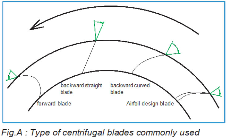
For a centrifugal fan, a forward curved blade produces more pressure, but operates with a lower efficiency than a backwards curved blade. For the industrial applications, the matter of efficiency involves a massive use of backwards blades. For a question of manufacturing cost, the blade is often plate or curved in a single plan and rarely “airfoil” designed to increase the efficiency.
Fan curve
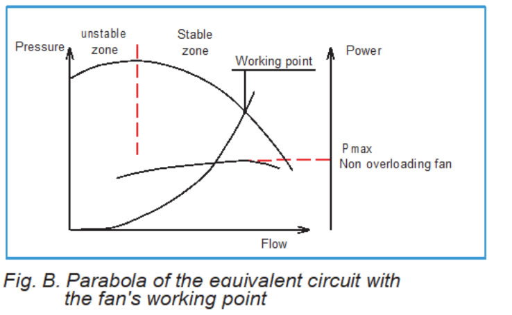
The fan is characterized by a pressure-flow and an absorbed power-flow curve, resulting from the bench test. For the fans with backward blades, the curve pressure-flow is in general first rising when the flow increase (this zone is unstable and might generate the “pumping effect”); then reaching a peak and descending continuously (this zone is called stable).
The curve absorbed power-flow is in general rising with the flow, and sometimes reach a peak before descending. In this case, the fan is called “non-overloading” because whatever the flow is, we will not exceed the installed motor power.
Working point of the fan
The working point of the fan on a circuit is the meeting point between the curve of the fan and the parabola of the pressure drop of the circuit.
Static, dynamic and total pressure
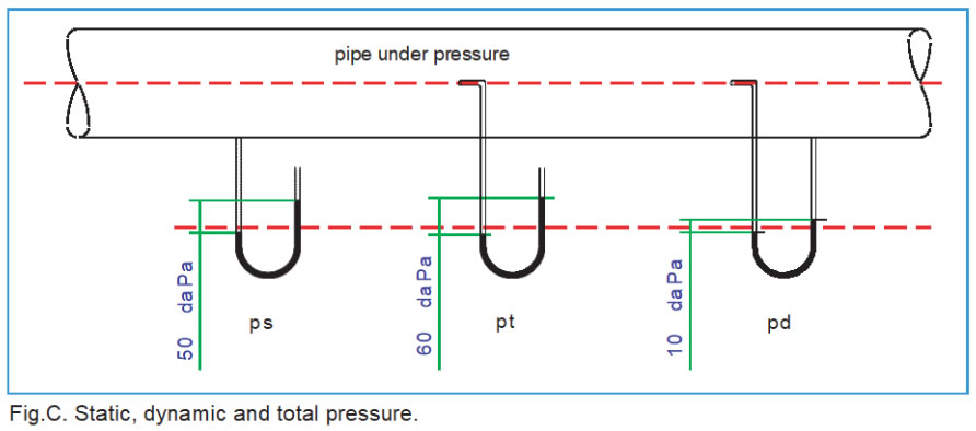
The static pressure is the one which is measured perpendicularly to the tank wall or in a pressurized pipe, and is independent from the air motion.
The dynamic pressure is the one which take birth from the air speed. It is the pressure pushing on you hand when you put it out of your moving car through the window. Another example is the pressure generated when you deflate a balloon with the air exiting by its tail.
The total pressure is the combination of both, static and dynamic pressure, including their sign (+or-).
These several pressure is expressed usually in Pa, DaPa, mmwk, or mbar.
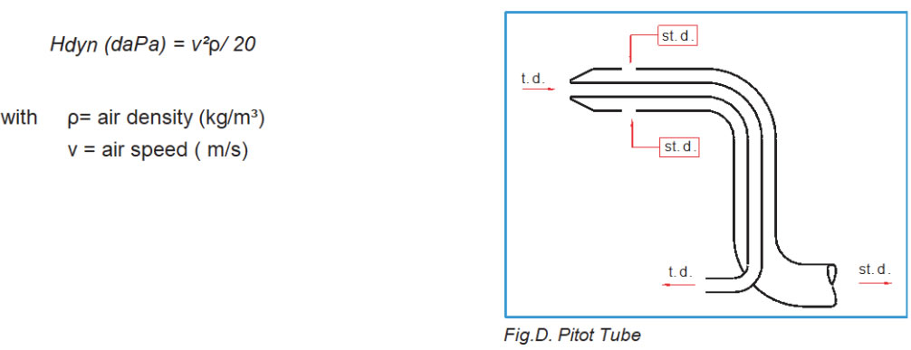
The dynamic pressure might be measured by the difference between total pressure and static pressure, bounding each to the plugs of a U manometer. This is the same principle used with the “Pitot Tube”. The dynamic pressure is the image of the air speed and therefore the flow.
Density
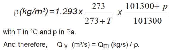
Under normal conditions, in others words by convention at 0°C and at the atmospheric pressure at sea level, the air density is equal to 1,293 kg/Nm³. For another temperature, or another pressure, it changes according the following law:
Consequence of the density variation with the pressure and the temperature, we must take into account this variation for the hot fluids, and also during the sizing of a fan operating at altitude. Furthermore, in this specific case, because of a lower air density, the cooling of the driving motor is less efficient, and we must in general, declassify it.
Pressure drop
The pressure drops of a circuit are usually proportional to the square of the flow and are a parabola of the second degree crossing by the origin in a system flow-pressure. They are expressed as following
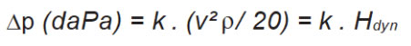
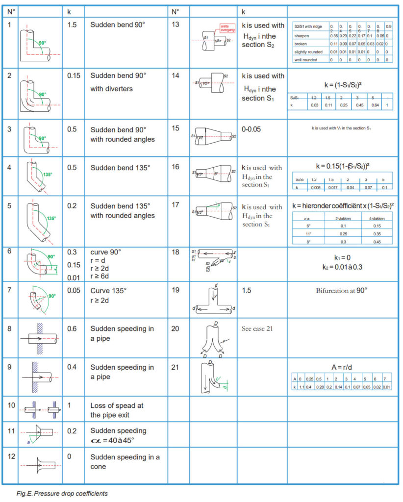
Within: k is a coefficient relative to the type of circuit accident.
The parabola of the equivalent circuit is then the sum of each particular parabola with the various pressures drops met on the circuit with occasional accidents (bends, enlargement section, …) or devices (filters, heat exchangers…)
Absorbed power
The absorbed power at the shaft is equal to the useful output power supplied to the fluid, divided by the efficiency of the fan.
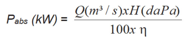
In order to calculate the absorbed power at the electrical grid, we should include the transmission, the electrical motor and the eventual variable speed drive efficiencies into account.
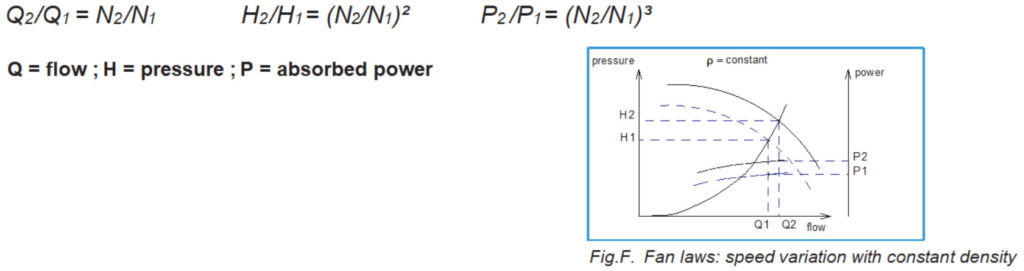
The fan laws
1/ Without any change in the circuit of the fan and with the same density, if we modify only the rotational speed of the fan passing from N1 (RPM) to N2, we will have new working conditions according the laws below:
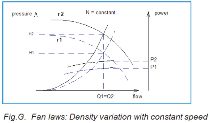
2/ In the same circuit with a cosntant speed, if the fluid changes from the density ρ1(kg/m³) to ρ2
- the volume flow do not change: Q2/Q1 = 1
- the pressure drop, as well as the pressure generated by the fan, change in the volume flow ratio: H2/H1 = ρ2/ρ1.
- the absorbed power vary in the density ratio: P2/P1 = ρ2/ρ1.
- the efficiency of the fan do not change
- the working point moves vertically.
Fan’s noise
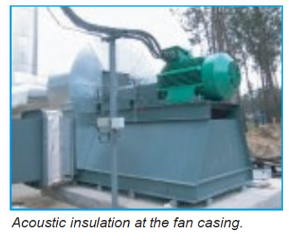
The fans are noisy machines in the need of an acoustic treatment, by the insulation of the casing and/or installation of a silencer at inlet/outlet
Pressure and power sound levels.
The ear is sensitive to the pressure variations of the air generated by sound vibrations. In the same way, the microphone of a sonometer measure the pressure sound level applied on its membrane.
The levels of pressure sound level (Lp in dB) are always expressed according a distance from the source. On the other side, the power sound levels (Lw in dB) are independent of the distance and, in the case of a source emitting uniformly in all directions, they might be calculated multiplying the pressure by the sphere area, with a radius equal to the distance of measurement of the pressure sound level regarding the source.
If P = the pressure sound level in W/m², W = the power sound level, and r = the radius of the sphere, centered on the source with the external area passing by the measurement point,
We get, P = W/4p r² and, expressed in dB, Lp = Lw + 10.log(1/4 pr²) with r expressed in m.
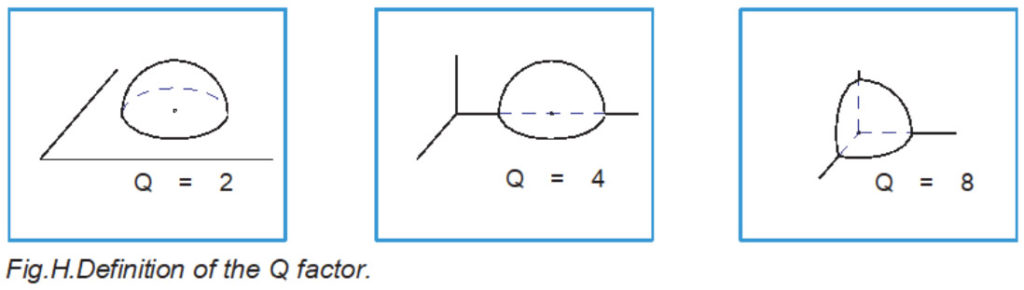
If the noise source has a directional effect, it will emit a total power W, but not anymore in an isotropic model through a sphere. We will therefore take into account a directional Q factor equal to 2 for a free field source on the ground, 4 if the source is placed near a reverberant wall and 8 if it is placed on a corner made the ground and 2 reverberant walls.
We get then, Lp = Lw + 10.log(Q/4 pr²).
Consequence of the formula above, we can calculate what will be the noise when we change the measurement distance and that we switch from distance r1 to r2.
Lp2 = Lp1 +10.log(r1²/r2²) = Lp1 + 20.log(r1 /r2 ).
Particularly if we double the distance Lp2 = Lp1 – 6.
Weighting curves
The physiology of the human ear is particular. The ear will not detect as uncomfortable two noises at the same pressure level but at different frequencies.
In order to compare the different noise troubles, we should weight the several pressure levels according the sensitive frequencies for the human ear.
We use often the A weighting curve that you can find below:
| Average frequency of octave band | Hz | 63 | 125 | 250 | 500 | 1k | 2k | 4k | 8k |
| Weighting A | dB | -26 | -16 | -8.6 | -3.2 | 0 | +1.2 | +1 | -1.1 |
Acoustic levels composition
To obtain the global noise level of an acoustic spectrum, we must add logarithmically the Lpi emitted in each octave band.
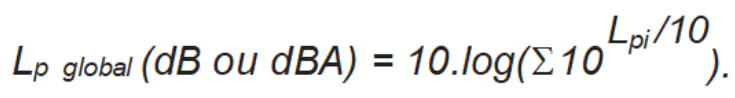
We can also use the formula below in order to know the resulting noise level emitted by several sources. We will therefore observe that, the gap of noise level between the two sources will outpass 10 dB, the sum of the two noise levels will give a non-significant correction regarding the noisiest level. We say that the noisiest level is “masking” the lower level.
Especially, if Lpw is the noise of a single fan, the noise resulting of two identical fans operating side by side, will be 3 dB higher than the fan operating alone. Indeed:

We can obviously extrapolate to “n” fans. If they are not identical, we will first operate the logarithmic sum of the n band level, frequency by frequency band, and we will recompose the spectrum of resulting values in order to get the global level.
Free and reverb field
The formulas above are applicable when in free and non-reverb field. If we are in a room, we are facing obstacles reverbing the sound waves and influencing the measurement by indirect wave addition. An acoustic study of the room by a specialized company will be necessary in order to calculate the average absorption coefficient α, the room volume, the surface of the walls and the reverbing time of the room. This study will help to define the noise level acceptable of each machine separately in order to that the resulting noise level will be lower to the requested noise limit (usually 85 dB(A)).